1. What is Optimisation?

• The concept of producing the best possible result with the available resources
• Optimisation is the process of minimising or maximising something
• It is an iterative process
• E.g. looking for the maximum point on the mountain:

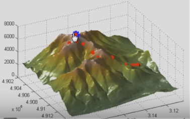
2. The Physical Problem

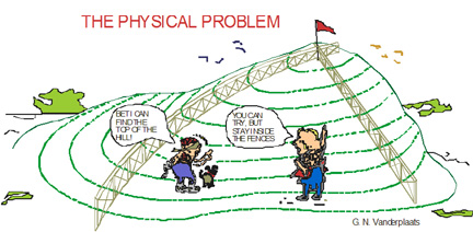
• One boy bets the other that he can locate the top of the hill blindfolded
• The other boy agrees but asks the first boy to also stay inside the fences
• Translating this situation into an optimisation formulation, we see that the objective is to find the highest point on the hill
• Therefore the objective function is the height achieved by the first boy with respect to his original position
• The variables of this objective function could be longitude and latitude (x and y), defining the position of the boy
• The constraints are that the boy has to stay inside the fences
• It is possible to define this problem mathematically

3. The Engineering Problem

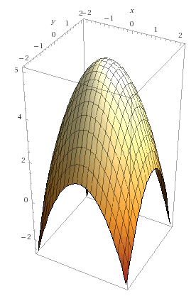
• Our objective is to find the highest point on the hill, so our objective function would be a curve (or 3-D surface) defining the hill itself
• We can define a function for the hill like so:

• Mathematically the hill is a graph in 3 dimensions; x (= X1), y (= X2) and z (=Y)
• It could look something like this:

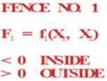
• Next, we need to define our constraints which in this case would be two functions representing the two fences on the hill

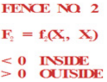
4. Formulating the Problem

• Maximize the objective function:

• Subject to the constraints:

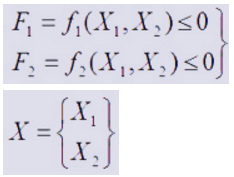
5. The Optimisation Process

• The optimisation process can be broken down into:
  • Find a search direction that will improve the objective (find the highest point on the hill) while staying inside the fences
  • Search in this direction until no more improvement can be made by going in this direction
  • Repeat the process, until no search can be found that improves the objective

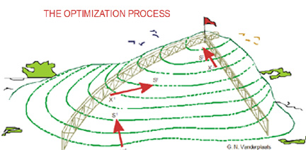
• There are many different algorithms available that search for the ‘optimum point’, each with a different method of getting there.
• Some are better suited to the problem than others as they require less iterations to find the optimum point; reducing time, memory & cpu usage
• This will depend on the problem itself:

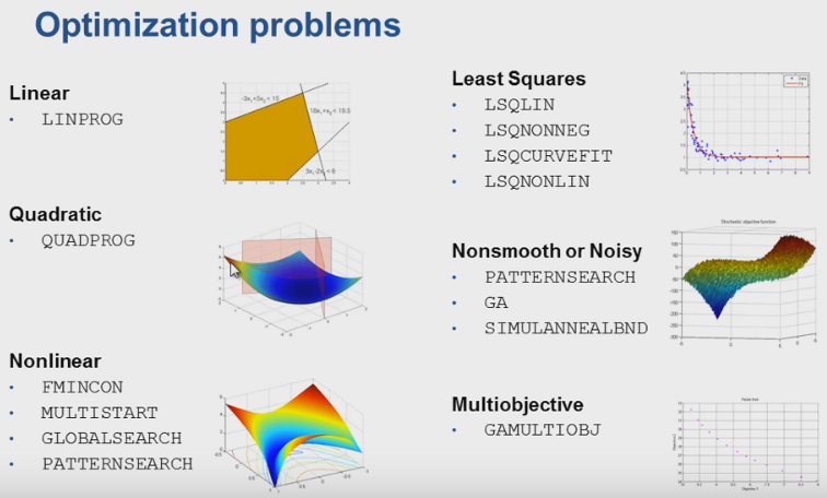
6. Optimisation Workflow

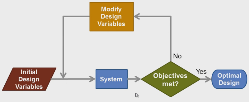
7. Benefits of Optimisation

• Finding better (optimal) designs
• Faster design evaluations
• Useful for trade-off analysis
• Non-intuitive designs may be found

8. Other Examples

• If we wish to design the internal combustion engine, the objective may be to maximise the combustion efficiency
• The engine may be required to provide a specific power output with an upper limit on the amount of harmful pollutants emitted into the atmosphere
• These parameters will serve as constraints for optimisation
• The variables that are allowed to be changed during optimisation may be the compression ratio, air-fuel mixture ratio, bore and stroke, etc
• You could also optimise:
  • The route of a delivery truck
  • A financial portfolio
  • Protein models

9. Final Project: A Simple Optimisation Problem

The Problem

• We need to enclose a field with a fence
• We have 500 metres of fencing material and a building is on one side of the field and so won’t need any fencing
• Determine the dimensions of the field that will enclose the largest area

Sketching the Problem

• In this problem we have two functions:
  • Objective function
  • Constraint function
• Sketching the situation will help us to arrive at these equations:

• In this problem we want to maximise the area of a field and we know that it will use a maximum of 500 metres of fencing material
• The area of the field will be the function we are trying to optimise and the amount of fencing is the constraint:

• Now we are ready to model and solve our problem in Julia

Setting Up Our Julia Environment

• Before we jump into the code, we need to install the relevant Julia optimisation packages
• Firstly we shall install JuMP; an algebraic modelling language for linear, quadratic and nonlinear constrained optimisation problems embedded in Julia
• Open the Julia application and in the command prompt enter:

• Next we shall install Ipopt; a nonlinear optimisation solver using the interior point algorithm to iterate to the optimum point

Create the Julia File

• Create a .jl julia file in a text editor – I have saved mine as “ example.jl “

Initial Comments

• First, it helps to write the problem in mathematical form as comments in the code
• This will help when coding the problem and also help others who may view your code to understand what you are trying to achieve

• From this it is clear we are trying to solve an optimisation problem

Import Packages

• Next we need to include the two packages (JuMP and Ipopt) in our example.jl file

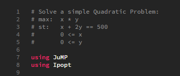
• Now all of the functions from the aforementioned packages are available to us when we run our example.jl script

Create a Model

• Next we need to define our Model, which we will name “ m “

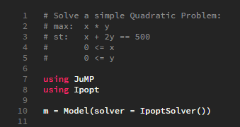
• Models are Julia objects and all variables and constraints are associated with a Model object
• Also, in the argument we state the solver we are going to use for this particular problem (there are many other solvers available – see here)

Define Variables

• Now we need to define the variables of our problem and their bounds
• The first argument will always be the Model to associate this variable with

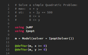
• As we can see from the comments (lines 1-5), clearly the variables are x and y and both have a lower bound of 0 (line 4-5)

Objective Function

• With JuMP it is very easy to define the objective function

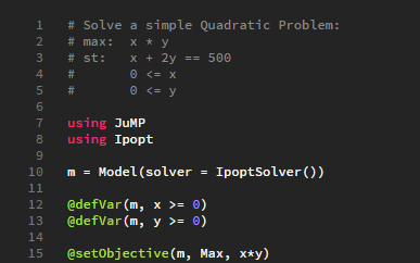
• The first argument will always be the Model to associate this function with
• The second argument is whether we are trying to find the minimum (Min) or maximum (Max) optimal solution
• Finally the third argument is the objective function itself

Constraints

• As with the objective function, JuMP makes it very simple to define constraints

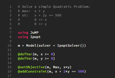
• The first argument will always be the Model to associate this function with
• The second argument is the constraint
• It is worth noting that we can define multiple constraints in this way

Print Model

• When we run our ‘example.jl’ Julia script, it would be useful if we could see what our model looks like before the optimising (solving) process begins

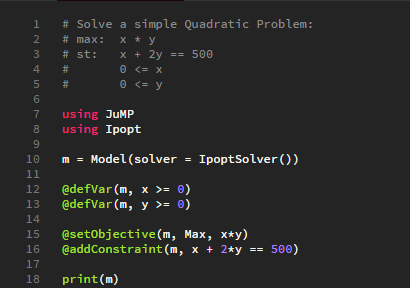
• The print function is defined for models and allows us to see our model looks like in a human readable format
• When we run our example.jl file the model will look like this:

Solve

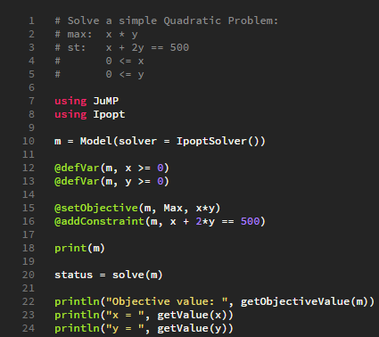
• Models are solved with the solve() function
• This function will not raise an error if your model is infeasible – instead it will return a flag
• In this case, the model is feasible so the value of status will be :Optimal

Print Results

• Finally we can access the results of our optimisation
• Getting the values for the objective function and x & y variables is simple

Solution

• Now we are ready to save and run our ‘example.jl’ script
• Open a Julia command prompt

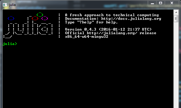
• Locate the directory where ‘example.jl’ is saved using cd()
• Remember to use “ \\ “ when entering the directory

• Now to run the ‘example.jl’ script we use include()

• Finally we have our results

Results

• The original question was to determine the maximum possible area of the field given we have 500 metres of fencing material and there is a building on one side of the field so won’t need any fencing

• We can see from running our ‘example.jl’ Julia script that the maximum area of the field is 31,350 m²
• We can clearly see the values for x (250 m) and y (125 m) satisfy the constraint x+2y = 500